The dashboard has nine layers. Turning them all on at once is overwhelming — and not useful. This guide walks through the order that actually tells the story: terrain → drainage → flood-prone zones → orientation → population → validation against real history. Five steps to get the picture; two more to compare alternatives.
Start with terrain alone
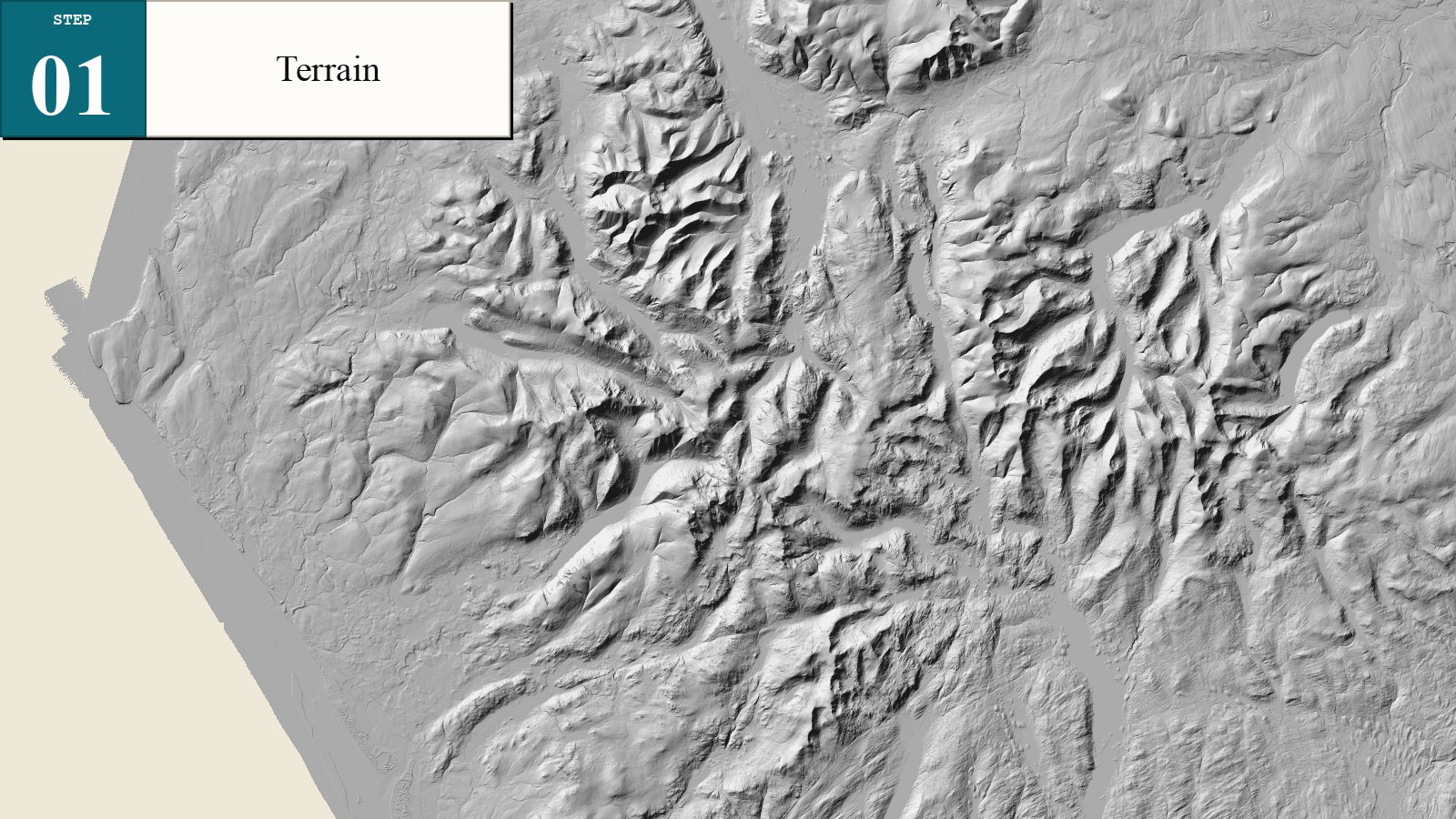
OFF: everything else
The bare relief. EA 1 m LIDAR Composite rendered as a north-west-illuminated hillshade. See the shape of Cumbria — Skiddaw + Bassenthwaite north; Buttermere + Wasdale west; Scafell central; Helvellyn + Ullswater east; Eden basin to the north-east; coastal plain west.
The dark voids around the edges are where LIDAR doesn't cover — Solway Firth (NW), Irish Sea (W), Pennine fringe (E).
Add HAND — where water naturally collects
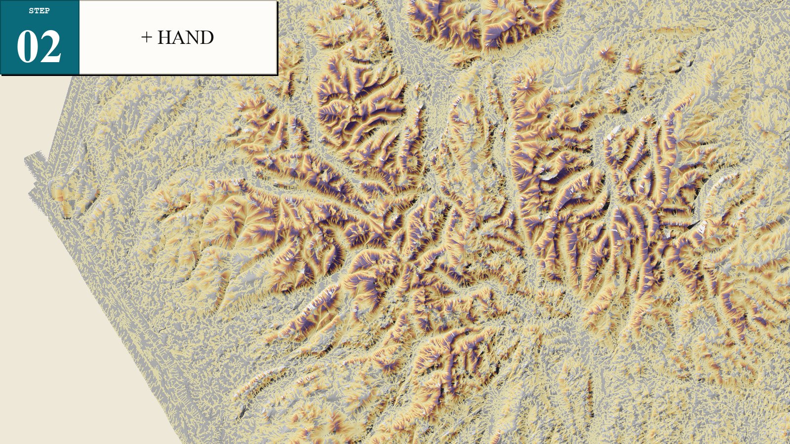
OFF: everything else
HAND (Height Above Nearest Drainage, Nobre et al. 2011) tints each cell by how high it sits above the nearest stream.
Yellow valleys = at or near channel level (potentially flood-prone). Orange / brown = mid-slopes. Purple ridges = upland, hydrologically safe.
Channel-init threshold: 0.025 km² (2.5 ha) — chosen empirically against real-world river networks; defensible for UK flood mapping.
Add lakes — anchor recognition
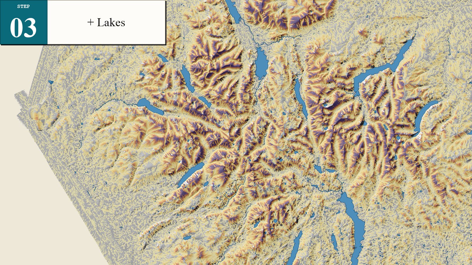
OFF: everything else
Add the lakes. Bassenthwaite, Derwentwater, Buttermere, Crummock, Wast Water, Loweswater, Ullswater, Thirlmere, Coniston, Windermere — instantly the map becomes readable for anyone who knows Cumbria.
Source: OpenStreetMap natural=water polygons (ODbL). 2,209 lake + tarn polygons within the extent.
Add towns — population context
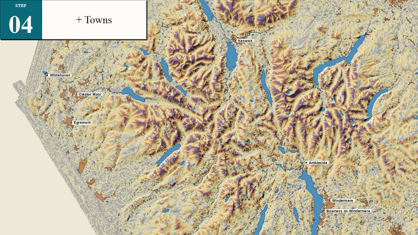
OFF: everything else
Now the question stops being abstract. Cockermouth, Keswick, Workington, Whitehaven, Egremont, Penrith, Kendal, Ambleside, Windermere, Bowness — the towns at risk.
Brown polygons = OSM residential/commercial/industrial footprints (built-up land). Black-edged dots = named place centroids; major towns labelled at all zooms, villages appear when zoomed in.
Add historic floods — does the prediction match reality?
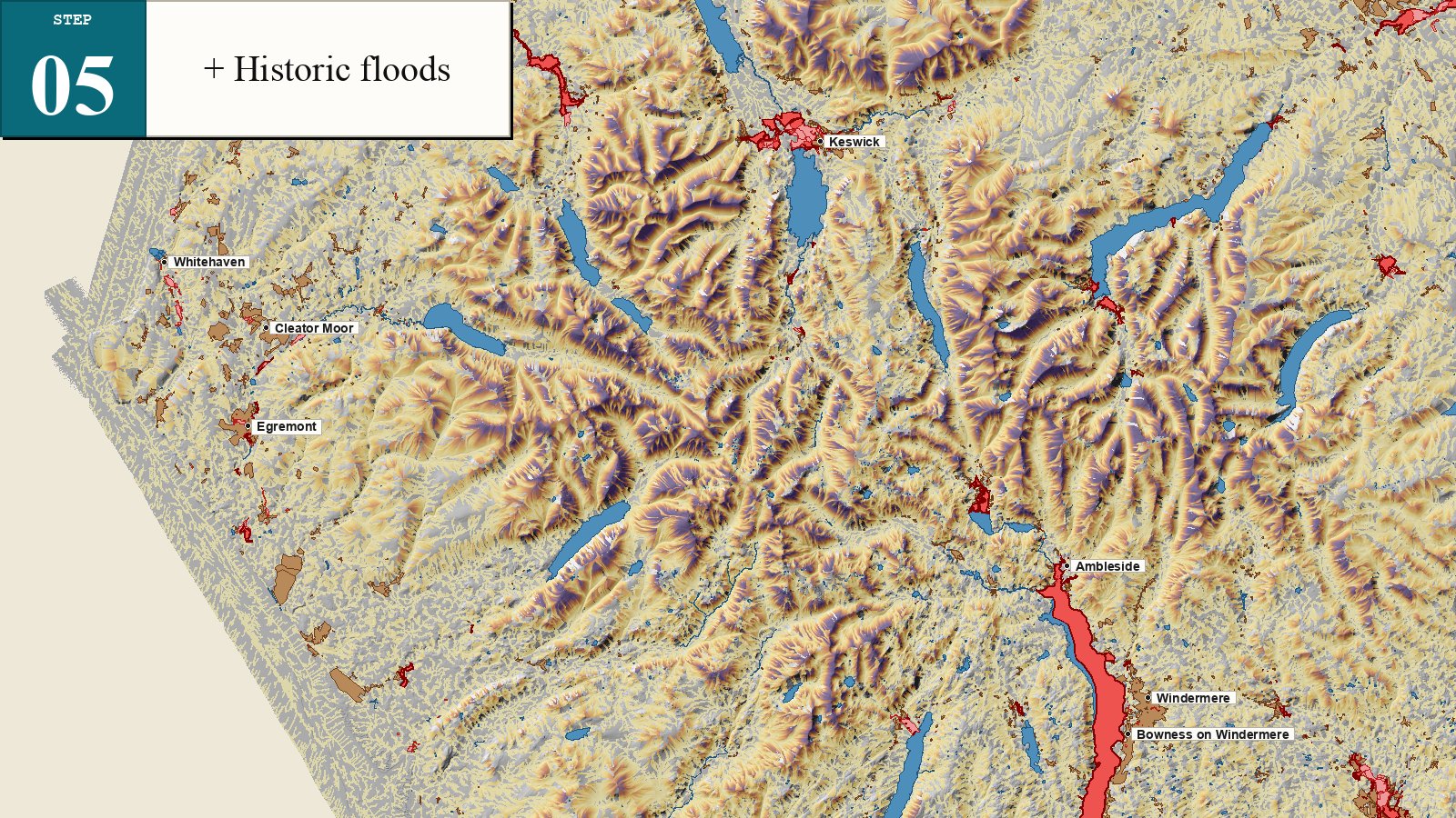
EA Recorded Flood Outlines (OGL v3) — actual flooded extents from the EA's records. 901 polygons across 348 events within Cumbria, including:
• Cockermouth November 2009 (the catastrophic flood that triggered the EA's modern flood-defence rebuild)
• Storm Desmond December 2015 (Carlisle, Keswick, Kendal — 65 flooded areas in one event)
• Storm Dennis 2020, Storm Ciara 2020, Storm Henk 2024, Brigham 2025
Major 2009 + 2015 events are styled darker red and slightly more opaque. Hover any polygon for event name and date.
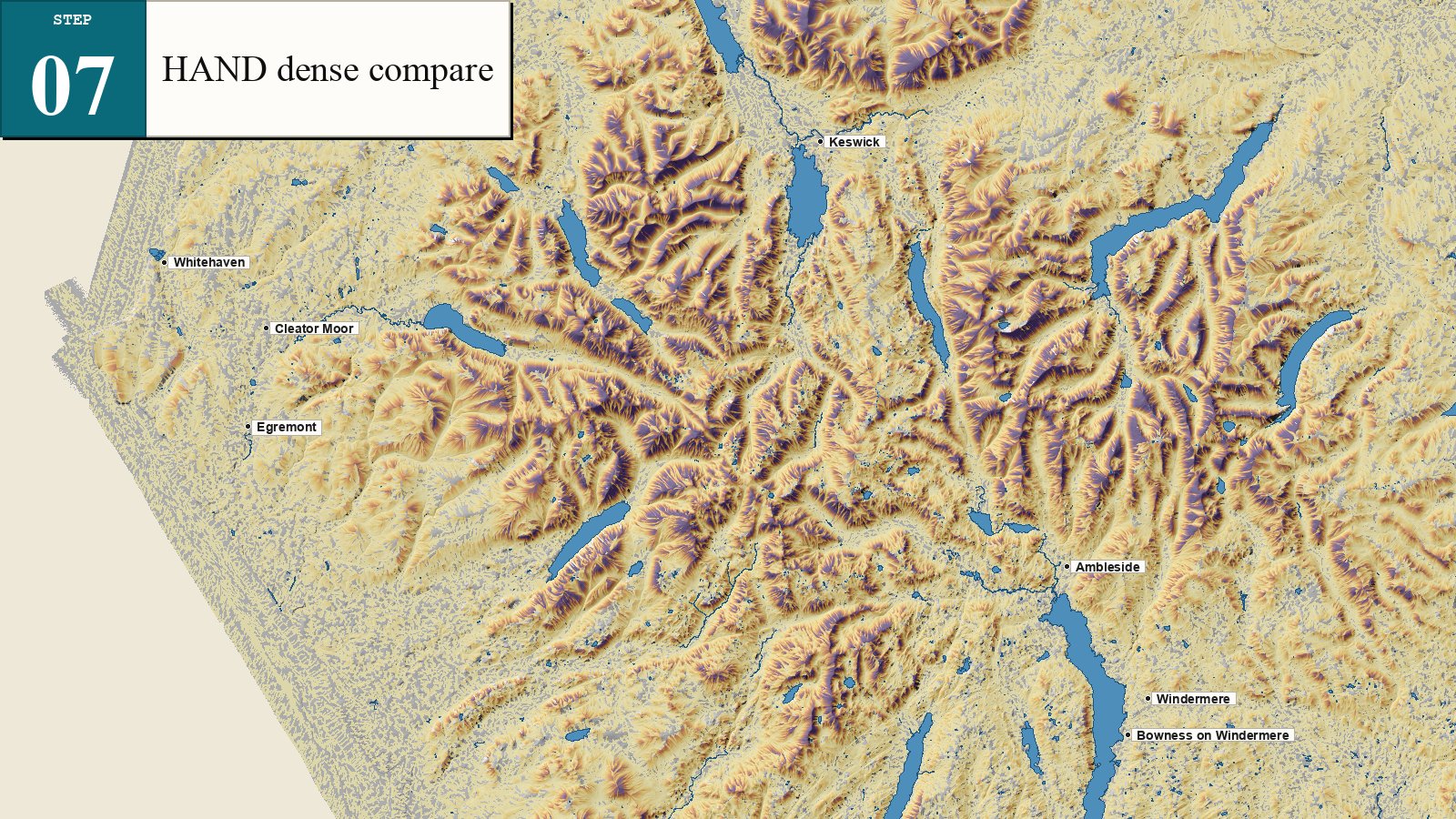
Compare HAND densities (advanced)
Lower the channel-init threshold from 0.025 km² → 0.01 km². More streams, more cells with HAND (45 % of land vs 35 %). The trade-off: small drainage ditches start to be counted as channels, so some areas of the lowlands are visibly over-extracted.
Toggle between them to see the genuine uncertainty in WHERE the algorithm draws the line.
Streams — what HAND is computed from
OFF: HAND, everything else (so you can see the channels clearly)
The extracted drainage network. Every blue line is a cell where the flow accumulation exceeds the 0.025 km² channel-init threshold. The blue web you see is what HAND measures distance to.
Compare against your mental map: Eden, Cocker, Derwent, Greta, Kent, Lune, Esk, Mite, Calder, Ehen, Bleng — all there.